Part 2: How Our Data Warehouse Used to Work — and Why We Needed to Change

Part 2: The New Data Layer — Vatico Training

✓

The Old Layer
(Part 1 — Done)

The New Layer
(You are here)

In Part 1, we covered how Vatico’s original data warehouse worked — a flat collection of ~400 purpose-built tables — and why that approach started to break down as the business grew. In Part 2, we walk through the new architecture: what each layer does, why it was designed that way, and how it directly solves the problems we ran into before. No heavy technical background needed.

A Quick Recap: The Problems We Were Solving

Before diving into the new design, it helps to keep the symptoms from Part 1 in mind. Every decision in the new architecture is a direct response to something that was painful before.

What we were trying to fix from Part 1

Symptom 1 — Too many tables with no clear map. ~400 tables, each built for one specific purpose. New analysts spent hours figuring out which table was the right one to query. It worked in the past because we needed to get things done quickly, but it became unsustainable as the business grew.

Symptom 2 — Every new request meant a new table. Accumulated high maintenance risk, and changes in one table could silently break others downstream.

Symptom 3 — No native visibility. With no standardised structure, monitoring data freshness across 400 differently-synced tables was extremely hard without external tools.

Evaluating these symptoms against our core data requirements (Effective, Reliable, Rapid) reveals the root problems:

The Root Problem — Failing Core Data Requirements (Effective, Reliable, Rapid):

• Effective: The old stack was still functional (it got things done), so effectiveness was okay.
• Reliable (Major Problem): Pipelines became extremely hard to maintain or upgrade as workflows evolved. Transformation logic was scattered everywhere, requiring tedious QC — and human errors still slipped through (e.g., a simple typo in one query where order status was typed as 'eturned' instead of 'returned', causing sale orders to be misclassified).
• Rapid (Major Problem): High architectural complexity killed iteration speed. Having to run tedious manual QC on every script meant development was no longer rapid, as moving fast carried a high risk of breaking critical components.

The new architecture addresses these root problems by establishing clear, standardized layers — ensuring that changes are scoped predictably and updates don’t break existing pipelines.

Why Alibaba’s Architecture? The Case for Layers

The new design follows a layered data warehouse model popularised by Alibaba’s data platform team (the ODS → DIM/DWD → DWS → ADS pattern). Instead of a flat collection of single-purpose tables, data flows through a defined sequence of layers.

Why switch to a layered model? As a business scales, changes are inevitable. In a flat stack, any business logic change requires editing dozens of ad-hoc scripts. Alibaba’s model structures data into distinct tiers so changes can be executed cleanly at the exact layer where they belong.

Here is how the old flat approach compares to the new layered design when managing changes:

❌ Old — Flat Design

Build for the moment

Each new use case gets a new table. Transformation logic is duplicated everywhere. No clear boundaries. Changes require tracing and modifying scattered scripts.

✓ New — Layered Design

Straight forward changes

Requirements can change, but updates are localized to their respective layer: application-specific view changes only affect ADS; shared metric logic changes affect DWS; raw schema updates affect ODS / DWD.

Reference: DataWorks Data Modeling – A Package of Data Model Management Solutions

The Five Layers: What Each One Does

Think of building the data warehouse like baking a cake. You start with raw ingredients, and by the time you’re done, you have something people can actually eat. Each layer is a step in that process — you can’t skip ahead, and each one depends on the one before it.

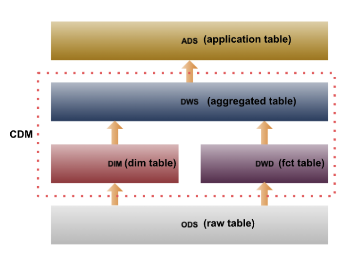
An example of the new data layer — ODS, DIM, DWD, DWS and ADS

The Five Layers — Vatico’s New Data Architecture

ODS Operational Data Store

An exact replica of raw data as it arrives from source systems (Webstores, CRM, Logistics Couriers, AWS Billing, etc.). No transformation or cleaning — a faithful copy for auditing and reprocessing.

Real table examples from our warehouse:
ods_api_woocommerce_src_orders_di ods_api_tiktok_marketing_src_ad_insights_di ods_api_aws_cost_explorer_src_cost_and_usage_mi ods_file_amazon_src_settlement_summary_mi
Naming: ods_[source_type]_[source_name]_[source_separator]_[table_core_name]_[update style]

DIM Dimension Tables

• Reference dimension tables created from ODS tables.
• Note: Detailed Star Schema design for DIM & DWD is covered in the dedicated section below. Naming: dim_[data domain]_[entity]_[update style]

DWD Data Warehouse Detail

• Tables corresponding to specific business processes at atomic event granularity.
• Note: Detailed Star Schema design for DIM & DWD is covered in the dedicated section below. Naming: dwd_[data domain]_[granular level]_[update style]

DWS Data Warehouse Service

• Summary tables containing common aggregated metrics used across multiple analyses and dashboards.
• Built on top of DIM and DWD layers.
Real table examples from our warehouse:
dws_woocommerce_revenue_insights_daily dws_fb_marketing_spend_daily
Naming: dws_[data domain]_[granular level]_[aggregation period]

ADS Application Data Service

Application-specific output views tailored for specific dashboards, APIs, or reports without cluttering the underlying DWS foundation.

Real table examples from our warehouse:
ads_fb_marketing_spend_daily
Naming: ads_[data domain]_[granular level]_[refresh cycle]

Update Style Codes — what hi / hf / di / df actually mean

The two dimensions: how often it syncs, and how much it brings in. hi = hourly incremental — syncs every hour, grabs only new or changed rows
hf = hourly full — syncs every hour, replaces the entire table
di = daily incremental — syncs once a day, grabs only new or changed rows
df = daily full — syncs once a day, replaces the entire table

A (not real) example of Data Domains

You will have noticed that table names include a short data domain code — qc, ffm, and so on. These are not arbitrary abbreviations. Ultimately, the mappings may change by the time you read this blog. But the concept here is to shorten and use standardized names when referring to your data domains. E.g. qc for quality control. stg for Staging.

Domain Code	Full name	What it covers at Vatico
qc	Quality Control	models for quality control
stg	Staging	Raw data before processing, temporary storage for ETL processes
usr	User	Customer profiles, buyer information, registration data
pmt	Payment	Payment records, reconciliation data, COD transfers, Stripe, VNPay

Note: these are subject to change by the time you read this blog. so please ask your supervisor again on what is the appropriate domain code to use.

How DIM and DWD Work Together: Star Schema

To understand the shape of our warehouse, you need to know how DIM (Dimensions) and DWD (Facts) fit together using a Star Schema layout.

Fact Tables (DWD): Contain event data and metrics — what happened, when, and how much (e.g. order transactions, shipment events, payments).

Dimension Tables (DIM): Contain reference context — who, what, and where (e.g. customer info, product details, courier names).

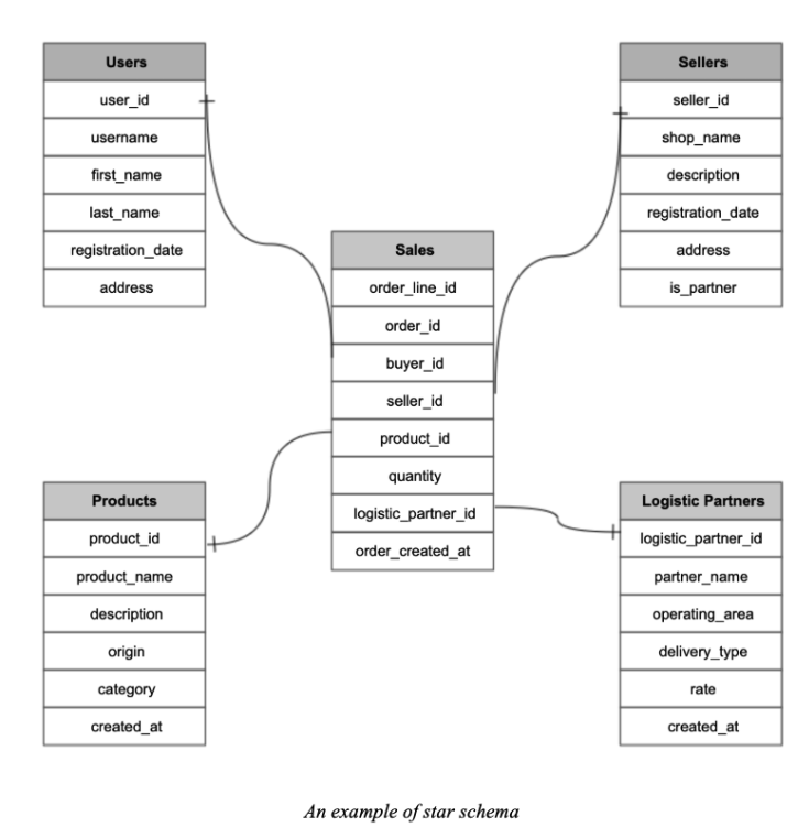
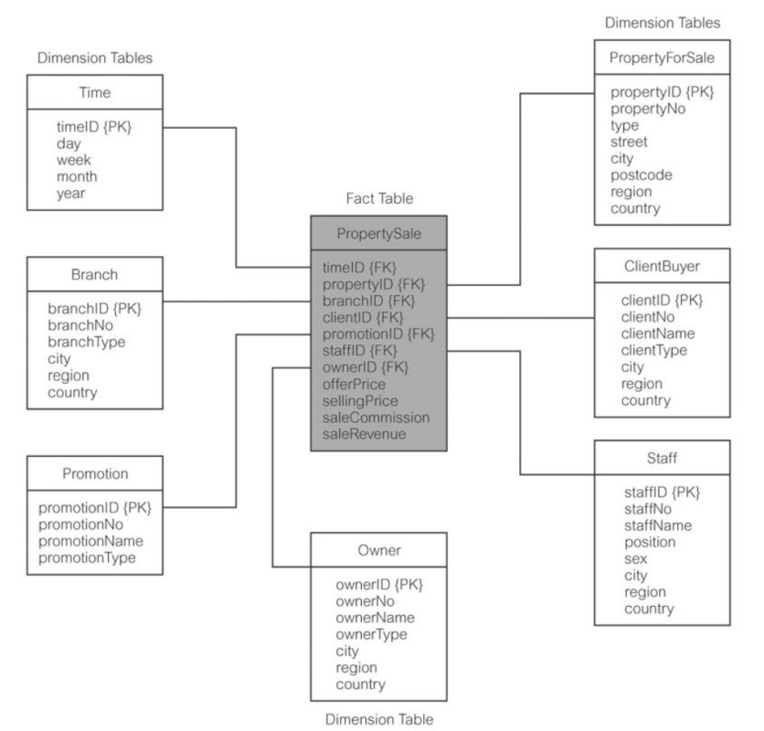
In a Star Schema, one central Fact table sits in the middle, surrounded by Dimension tables. Joining your DWD fact table to DIM lookup tables lets you slice metrics by product category, courier, or customer type without duplicating entity metadata.

Rule of thumb for interns: If a column answers “what happened or how many?”, it belongs in a DWD Fact table. If it answers “who, what, or where?”, it belongs in a DIM Dimension table.

Once you know the pattern, any table name tells its own story — no documentation needed.

Source: Alibaba Cloud — DataWorks Data Modeling

The “Which Table Do I Use?” Problem — Solved

In Part 1, we walked through a scenario where a new analyst spent three hours trying to find the right sales order table for a simple query. Let’s replay that scenario with the new architecture.

From Part 1 — the old experience

Your manager asks: “Can you pull the number of Sales Orders that were shipped in April, broken down by courier?”

You search for “sales order” and find 10 tables with the same words in the name. You pick one. The number doesn’t match the dashboard. Two hours later, you find the right table after tracing the lineage(upstream and downstream) and logic of the table.

The same question with the new architecture

Your manager asks: “Can you pull the number of Sales Orders that were shipped in April, broken down by courier?”

You know this is raw WooCommerce sales order data, so you look for the prefix matching raw source tables: ods_api_woocommerce_src_orders_di. One table, one clear source. You run your query and get the number instantly.

If you want a pre-aggregated view—like daily revenue insights—you look for dws_woocommerce_revenue_insights_daily. It’s already computed for you.

Five minutes, correct number, no archaeology.

What This Means for You as an Intern

When you are given a data task at Vatico, here is how the new architecture changes your workflow:

Your practical guide — how to navigate the new warehouse

Step 1 Identify the domain

Is the question about orders, shipping, payments, or customers? That tells you the domain code. This narrows the table list immediately.

Step 2 Pick the right layer

Need raw source data for backfill or audit? Use ODS. Need row-level detail? Go to DWD. Need pre-aggregated metrics? Go to DWS. Building or consuming a dashboard? Use ADS.

Step 3 Read the table name

The naming convention tells you everything: layer, domain, entity/process, and update cadence. dws_fb_marketing_spend_daily = summary layer, Facebook domain, marketing spend entity, daily refresh. No guessing needed.

One practical tip: if you are ever unsure which table to use, the layer prefix is always your first filter. Start with the prefix that matches your use case (dwd_, dws_, etc.), then filter by domain code (the abbreviation representing the topic, like usr for user or pmt for payments). You should almost never have more than a handful of candidate tables — and if you do, that is worth flagging.

Training Data